Alternative Data Regressor: V1
A Python Program to attain a linear regression of some alternative data against financial asset prices . A CSV file is the input. The output is the regression results.
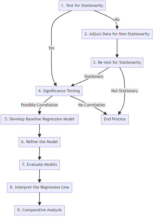
The provided Python program is designed to process time series data from a CSV file and execute a series of analytical steps based on a predefined decision tree. Key functionalities include:
Reading a CSV File: The user inputs the path to a CSV file, which the program reads into a DataFrame.
Stationarity Testing: It tests the time series data for stationarity using the Augmented Dickey-Fuller test.
Adjusting for Non-Stationarity: If the data is non-stationary, it applies a log transformation to stabilize the time series.
Re-testing for Stationarity: After transformation, it retests the data for stationarity.
Significance Testing: Conducts an Ordinary Least Squares (OLS) regression to test the significance of the relationship between the time series and a dependent variable.
Model Development and Evaluation: If a significant relationship is found, the program proceeds to develop a baseline regression model, which is then refined and evaluated based on its R-squared value.
Output: The program outputs the results of the stationarity tests, significance tests, and the R-squared value of the regression model.
import pandas as pd
import numpy as np
from statsmodels.tsa.stattools import adfuller
from statsmodels.regression.linear_model import OLS
import statsmodels.api as sm
from scipy import stats
import matplotlib.pyplot as plt
from sklearn.model_selection import train_test_split
from sklearn.metrics import r2_score

def test_stationarity(timeseries):
    # Perform Dickey-Fuller test:
    dftest = adfuller(timeseries, autolag='AIC')
    return dftest[1]  # p-value

def adjust_non_stationarity(data):
    # Adjusting for non-stationarity (example: log transformation)
    return np.log(data)

def significance_testing(X, y):
    # Perform significance testing (example: OLS regression)
    X = sm.add_constant(X)  # adding a constant
    model = OLS(y, X).fit()
    return model.pvalues

def main():
    # Load data
    file_path = input("Enter the path to your CSV file: ")
    df = pd.read_csv(file_path)

    # Assuming the time series column is named 'timeseries'
    timeseries = df['timeseries']

    # Step 1: Test for Stationarity
    if test_stationarity(timeseries) > 0.05:
        # Step 2: Adjust Data for Non-Stationarity
        timeseries = adjust_non_stationarity(timeseries)

        # Step 3: Re-test for Stationarity
        if test_stationarity(timeseries) > 0.05:
            print("Data is still non-stationary after transformation. Ending process.")
            return
        else:
            print("Data is stationary after transformation. Proceeding with analysis.")
    else:
        print("Data is stationary. Proceeding with analysis.")

    # Step 4: Significance Testing
    # Assuming another column 'dependent_var' as the dependent variable
    pvalues = significance_testing(df[['timeseries']], df['dependent_var'])
    if any(pval < 0.05 for pval in pvalues[1:]):  # Ignoring the constant's p-value
        print("Significant correlation found. Proceeding to model development.")
    else:
        print("No significant correlation found. Ending process.")
        return

    # Steps 5, 6, 7: Develop, Refine, and Evaluate Regression Model
    # This is a simplified example using OLS regression
    X_train, X_test, y_train, y_test = train_test_split(df[['timeseries']], df['dependent_var'], test_size=0.2, random_state=0)
    model = OLS(y_train, sm.add_constant(X_train)).fit()
    predictions = model.predict(sm.add_constant(X_test))
    print("Model R-squared:", r2_score(y_test, predictions))

    # Step 8: Interpret the Regression Line
    # This step is more analytical and depends on the specific model and data

    # Step 9: Comparative Analysis


if __name__ == "__main__":
    main()